
Calculating the fine structure constant, part 1
In agreement with quantum electrodynamics, and ab initio
In 1916, Arnold Sommerfeld discovered the fine-structure constant. The most recent experimental value is 𝛼 = 1/137.0359991(1). Since its discovery, no convincing explanation for the value of the fine-structure constant, which describes the strength of the electromagnetic interaction at low energy, has been given. Where does the number come from?
Understanding the value of the fine-structure constant requires going beyond the standard model of particle physics. As told in this blog already a few times (and in the preprint linked at the end), there exists a single fundamental principle, based on fluctuating strands of Planck radius, that reproduces quantum theory, quantum electrodynamics, quantum chromodynamics, the standard model with massive neutrinos, and general relativity, all without measurable deviations. Strands thus go beyond the standard model, but, at the same time, agree with all experiments.
Strands have the advantage that, in contrast to the standard model, they determine unique particle masses and coupling constants, of which 𝛼 is one. The fine structure constant 𝛼 describes the strength of electromagnetism. Its square root also describes, as Feynman tells, the probability that an electron absorbs a photon. The square root also describes the phase change that an electron acquires when it absorbs a photon. These statements are sufficient to determine 𝛼 with the strand model, as shown now.
Electrons have a phase because they rotate. The rotation of electrons, their spin, is proven by the Einstein-de Haas effect. If you do not know it, look it up. If you are bombarded with stupid internet memes claiming that electrons do not rotate, read about this effect to know how wrong they are.
Electrons rotate, but they are not spheres. Their spin 1/2 proves it. (Spheres have spin 0.) But also 𝛼 proves it: if electrons were spherical, they would not have such a crazy number as absorption probability. Or as a phase change. In short, we know that electrons are rotating, but also that they are not spheres. What structure do they have? Well, Dirac told us since 1929 that electrons are fermions, and that therefore they are tethered.
Particles are indeed tethered, as confirmed by Battey-Pratt & Racey in 1980 for matter particles. (Click for reading their paper.) Indeed, Battey-Pratt and Racey showed that a tethered matter particle automatically follows the Dirac equation. In simple words, the Dirac equation is due to tethers!
But what about the central part of the particle, the part that spins? What structure does it have? Is it a golf ball, like Battey-Pratt and Racey imagined? The answer given by the strand tangle model is simple: particles, space, and horizons are all made of strands/tethers. Nature consists of strands. The strands have Planck radius. As a result, the strands are unobservable: they are invisible. They have no mass, no tension, and no elasticity. But the effects of the strands are observable: the three dimensions of empty space, and the curvature of space is due to the many strands making up space. In addition, particles are tangles of strands. This explains both spin 1/2 and spin 1, depending on the type of their tangling. Furthermore, horizons are tight weaves of strands; this explains the entropy, the temperature, and the mass of black holes.
It turns out that the tangle geometry of electrons completely determines the value of 𝛼. More precisely, the fine-structure constant follows from the geometry of the following process:
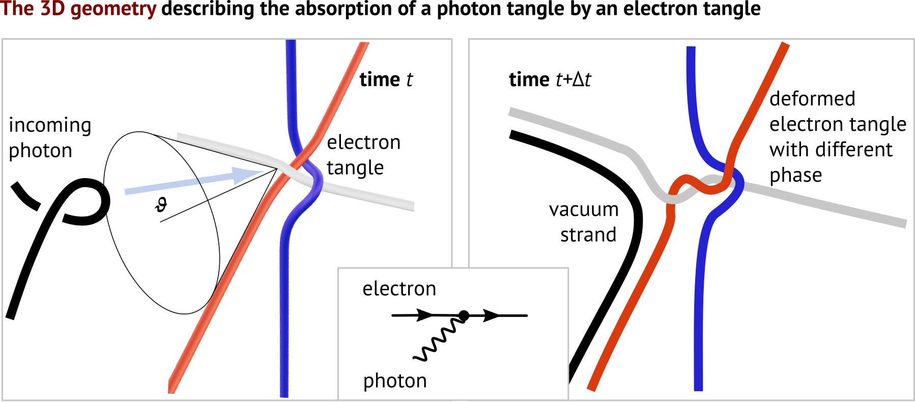
Taking into account the fluctuations of the strands yields the fine structure constant to full measurement precision, as will be shown in this and in the next part of the calculation.
The electron is assumed to be at rest. As a consequence, its 6 tethers are perpendicular. Each of the three outer crossings yields a charge e/3. (This also explains the charge of the quarks, which have a different structure, not shown here, and the charge of the W boson. Details are found in the preprint on the tiny theory linked at the end.) Given that the two images differ only by a few Planck times, spin and precession play no role.
The photon absorption probability p will depend on the incoming angle 𝝑. Because the full cone angle is a right angle on average, and because a photon arriving along the side of the cone does not affect the electron, whereas a photon along the cone axis has maximum effect, the general probability dependence for a fixed cone is
At the same time, the strands fluctuate. The cone will fluctuate in its cone angle and in its orientation. This yields a folding of the previous expression with a Gaussian distribution, leading to the probability
The cone orientation can have infinitely large angles with respect to the incoming photon, because the strands can wind up without limit.
The variance of the angle in one direction is the square of the average cone angle
Given that the incoming photon is described by an azimuthal and a polar angle, the total variance is twice this value. Finally, we need Feynman’s definition that the fine-structure constant is the square of the probability p. Together, this yields an initial approximation for the fine structure constant given by
This initial approximation differs from the measured value - 1/137.0359991(1) - by about 1.5%. This is not a good approximation, but it will get better soon, in the second part of this post series.
Note that this initial approximation was already proposed in 2004 by de Vries! He found it intuitively, without an underlying model. No other author ever thought about this approximation. Only de Vries, and nobody else, had the intuition to use it as the staring point for further improvements. As we will see in the next part of this calculation, de Vries also deduced, already in 2004, an improved expression for the fine-structure constant that still agrees with all observations today, 22 years later.
Note that fluctuating strands provide a model explaining de Vries’ initial approximation. The strand fluctuations lead to an expression for the fine structure constant that only depends on e (because of the Gaussian) and on 𝜋 (because of the 3D structure of the electron tangle).
As we will see in the next part, strands also provide the underlying model for all the improved expressions by de Vries: not only for his initial approximation but also for all the following ones. The fluctuations of the strands and the geometry of the electron tangle explain them. A literature search confirms that no other attempts to derive the fine structure constant from a Planck-scale model of particles in 3D exists. (However, there is one different, competing model: Singh’s octonion model also derives the fine-structure constant, though with a more involved and more abstract geometry, not in 3D.)
De Vries’ final formula is unique across the literature. The next part of the strand calculation of the fine-structure constant will increase the precision by taking into account virtual particles, which were neglected so far, and will yield a result for the fine structure constant that agrees with all experiments and that provides a test for all future measurements.
*
A technical reference is this new paper, from July 2026: https://zenodo.org/records/21467195
Strands allow to classify tangles and interactions with theorems from topology. To read more about the classification leading to the interactions with their gauge groups, as well as the classification leading to the elementary particles with their masses and quantum numbers, see the preprint https://www.researchgate.net/publication/397264142 on the tiny theory. Enjoy.
* * *